
Using consumer electronics analogies to demystify earthquake system specifications
The persuasive power of numbers is often used to try to summarise complicated systems into simple comparable numbers. 135dB, 2000V/m/s, 40Vpp – for seismologists with limited understanding of electronics, these numbers are not an intuitive indicator of seismic system quality or performance. Are bigger or smaller numbers better, or is it all relative, and does the specification even matter at all?
For example, you’d think you could judge the performance of an earthquake monitoring system based on a sensor’s “Sensitivity” value. It sounds like it must be the defining specification of an earthquake detector, right? Well, no. Sensors are just one part of an earthquake recording system, so you need to look at how components work together to get the true picture.
Using 32-bit technology to get quality 24-bit data

As well as being an earthquake observatory, the SRC is one of a handful of specialist companies that build seismographs (high speed digital data loggers that record very small analogue voltages) that are designed specifically for recording earthquakes. Modern earthquake data loggers use 32-bit technology for their analogue-to-digital converters (ADCs), but typically only 24-bits of the output is noise-free, so information is usually stored at this resolution, which also aids in data compression. 24-bit resolution means that we can see signals almost as small as one 17-millionth of the full range.
To use an analogy, a seismograph can be thought of as a digital camera with a zoom lens. Imagine having a 17 megapixel camera with different lenses – a wide angle lens allows you to capture a wide field of view, and a zoom lens you see more detail, but only in a portion of the scene.
Most seismographs come fitted with a “wide angle” (think zoom of x0.125) input that allows recording of a 40 Volt (±20V) range by the 5 Volt ADC. This means that in theory the smallest detectable difference between two data points is 2.4 microvolts. The direct (x1 zoom) ADC input allows for 300nV increments to be visible, or you can increase magnification by up to x64 zoom to look at even smaller voltage changes.
Like digital photography, you can’t capture everything you can see in a single photo – you’re still limited to the 17 megapixels. You have to trade between the level of detail and the scope of image. This is the current limitation of digital recording technology, but like your modern multi-lens smartphone, a multi-channel recorders can record both wide angle and zoomed images at the same time.
Sensor “Sensitivity” doesn’t mean Sensitivity
The “Sensitivity” of an earthquake sensor describes its analogue voltage output, which is defined in “Volts per metre per second” (for velocity sensors) or “Volts per g” (for acceleration sensors). A sensor will also have a maximum output voltage.
If a seismometer has 1500V/m/s sensitivity and a ±20V maximum output, the maximum signal that you can record is 13.3mm/s. This is known as the “clip level”. You could achieve the same clip level with a 750V/m/s sensor at a clip/zoom level of ±10V, or about 14mm/s for a 350V/m/s sensor at a ±5V clip/zoom level.
So, a 1500 V/m/s sensor is not necessarily better than one with 350 V/m/s – it just means that its output is suited to a particular “lens” (to continue with the camera analogy) to achieve a specific result. A 350 V/m/s output sensor can achieve similarly cropped picture with a suitable recorder zoom setting.
As such, “Clip Level” and “Sensitivity” do not tell you how sensitive the sensor is. In camera terms, it just tells you how big the subject can get, which can help you decide what angle lens you need to use to be able to capture the whole picture.
Now that you know which lens is needed to capture the biggest parts of the picture, the quality of your image comes down to how much detail is in your subject. Are you seeing distinct details in every pixel, or is it a noisy grainy image when you’re zooming into your digital photo album? This will come down to the noise level of your seismic sensor. Most sensors have a lower noise level than that of your recorder’s “camera”, but some do not.
Dynamic Range – the Bit’s the Limit
Ground motions in excess of 2g (twice the acceleration due to gravity) have been recorded from the largest of nearby earthquakes. If this is the upper end of dynamic motion from earthquakes, how far down the range of ground motion can we go and still detect vibrations? At the quietest locations on earth it is possible to see vibration levels of less than a billionth of the force of gravity. This “dynamic range” (from the strongest to weakest of detectable motions) is measured in decibels, and equates to about 200dB.
Dynamic range of an analogue earthquake sensor represents the motion from the clip level to the noise level, but because the noise level of a sensor varies with frequency, the widest dynamic range is often stated to present the most favourable number. As such, noise level and dynamic range are closely related. Low cost acceleration sensors have ranges of around 100dB, whereas high tech velocity sensors can have ranges in excess of 160dB.
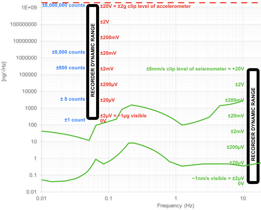
Each bit of a digital system represents about 6dB, so a noise-free 24-bit system has a theoretical dynamic range of 144dB, which means that even the best recorders can’t record the full dynamic range of the best sensors. As you can see in the diagram above, this is why you need two sets of recording systems to cover the full dynamic range of ground motion.
A single bit of digital noise (1 count in 17 million) reduces a recorder’s dynamic range to 138dB, and 2 bits of noise results in 132dB of dynamic range. This small amount of digital noise can have a massive effect on a specification that is perceived as a measure of recorder performance, but the real-world implication is not as dramatic. Often recorder dynamic range is averaged and other dB numbers are quoted, but most have 1-2 counts of digital noise in typical operation modes.
The Noisy Earth
The Earth is always vibrating, and some places vibrate more than others. Urban environments are inherently noisy, as are coastal locations where ocean waves continually crash onto the land. Reclaimed land and relatively loose surface conditions can also be noisy, but there are some very quiet places on earth where we can measure the natural vibrations of the Earth at various frequencies.
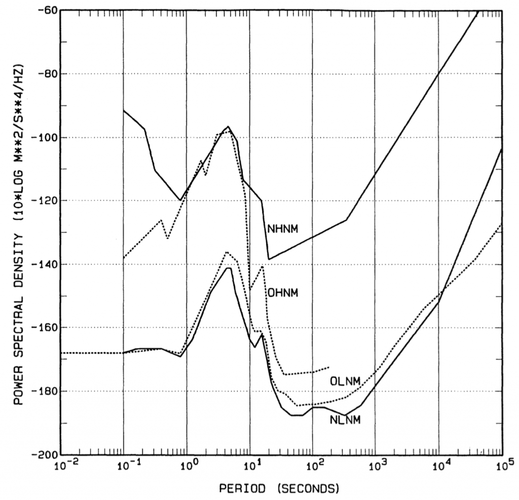
Because of the frequency-related (spectral) variability of seismic noise, it is impossible to define a location’s noise level as a single number, so it is often presented on an amplitude-frequency graph. The relative noise is visualised by models developed by Peterson, where the NLNM (New Low Noise Model) is a representation of the spectral noise at the quietest seismic stations on earth, and the NHNM (New High Noise Model) are the spectral noise levels in an urban environment.
The ability of the sensor to detect small levels of motion is also frequency-dependent. Some sensors will output consistent voltages at very low frequencies of motion, and others will only do so at higher frequencies. Sensors that have a consistent signal amplitude over a wide band of frequencies are know as “broadband” sensors, and in terms of earthquake monitoring this typically covers long period signals from at least 30-seconds (0.033Hz) to frequencies of at least 50Hz.

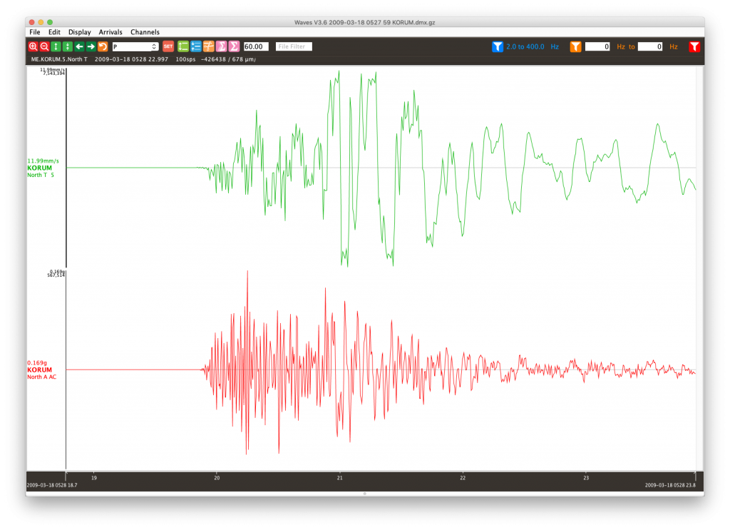
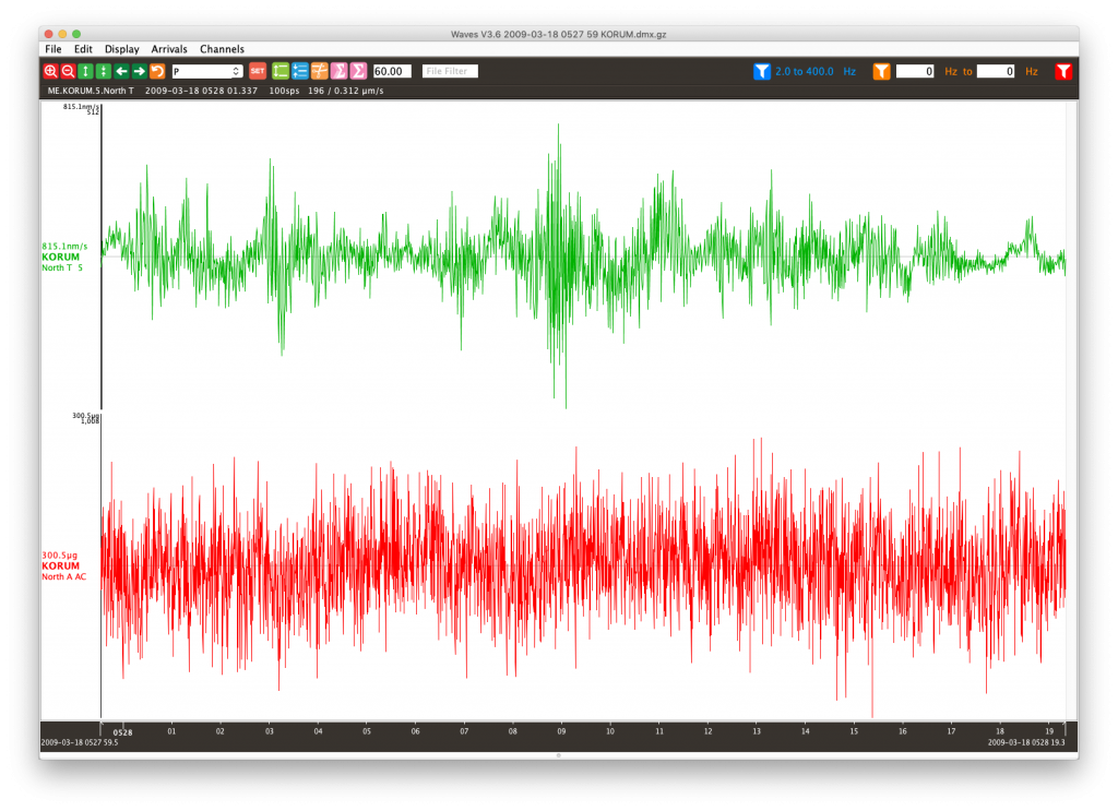
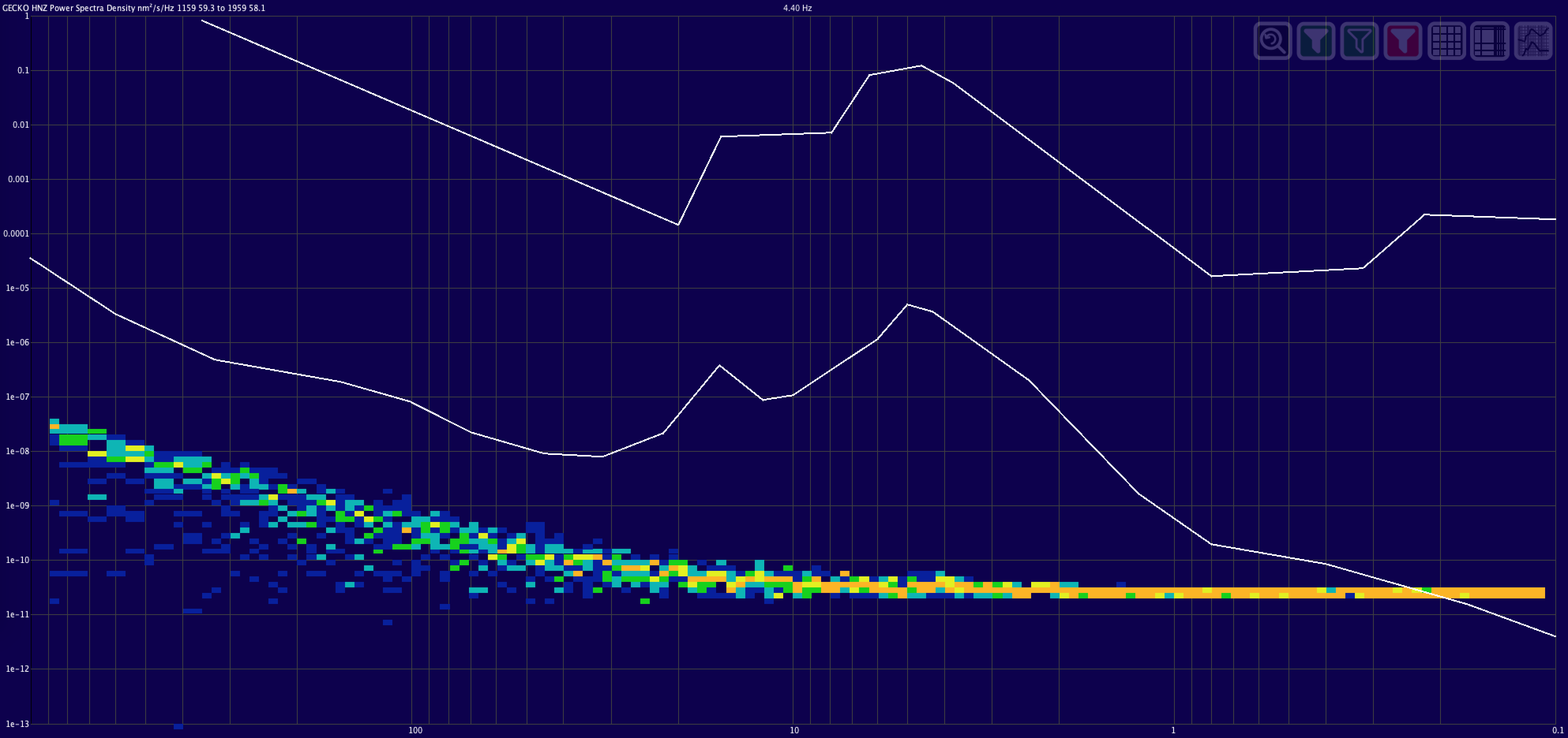
If you are interested in monitoring very small seismic signal levels (those around the NLNM) the sensor noise and the ambient noise at the station is usually a limiting factor. The recorder needs to be set up with the appropriate “zoom” level for the sensor so that the recorder is not limiting signal detectability. This can be seen below, where the self-noise level of a Gecko recorder set up to record a low noise seismometer is below the low noise model from 1000 seconds to where it crosses the NLNM at 5Hz.
Compare this to the noise level of one of Australia’s national network stations that is located in a quiet underground vault. It uses a very low noise 1500V/m/s Streckeisen STS-2 120-second seismometer. We know this sensor can detect even smaller signals, so this plot shows the station’s noise level from a period of a few hours of sampled data.
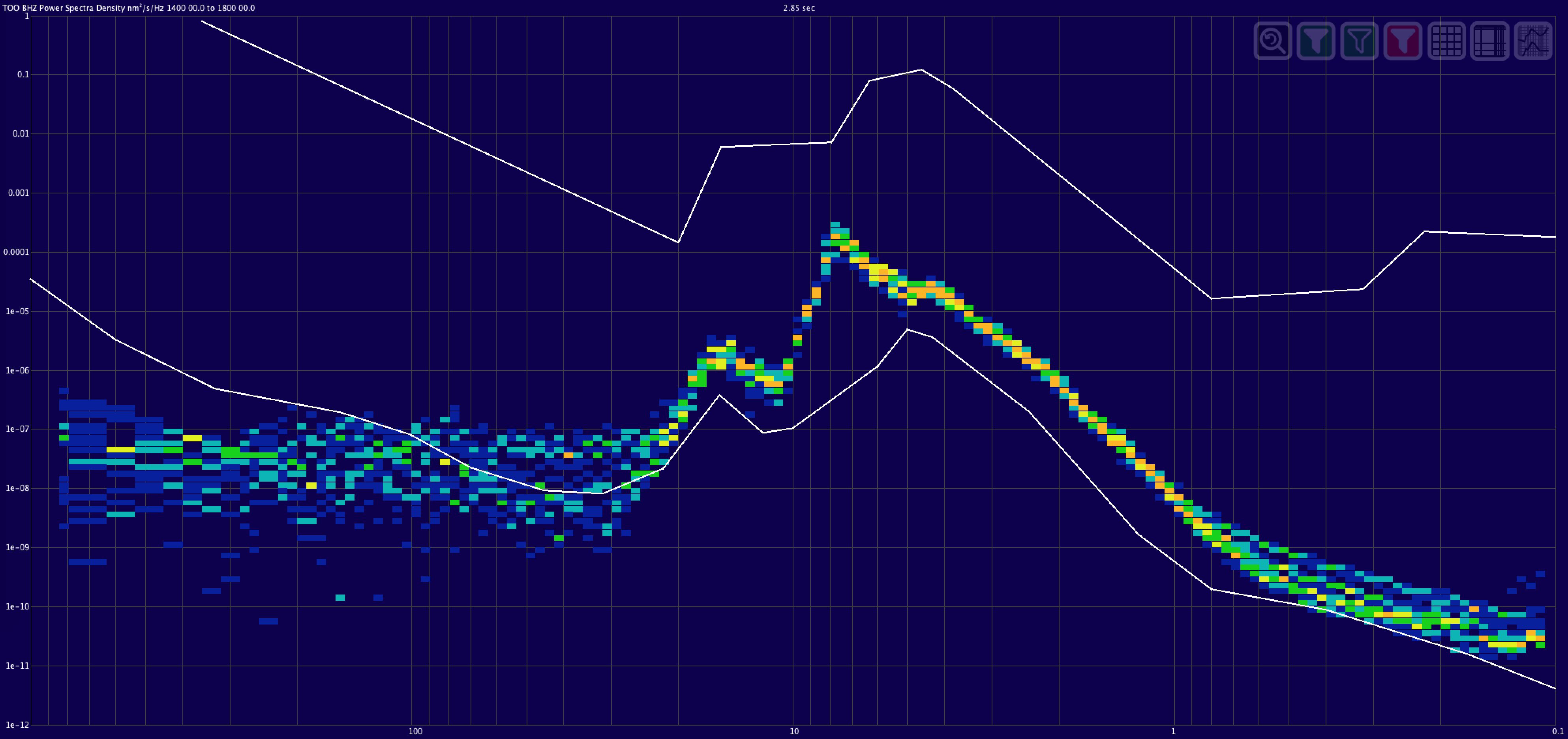
Noise levels at most non-permanent seismic stations are in the middle of the noise model range (between the NLNM and NHNM lines, so having a sensor that can detect much lower signal levels may not be worth the added expense. Selecting the right sensor means looking at where you are going to install it, and what you want to record. For earthquake monitoring, you generally want to use a sensor that has a noise level in the range between the NLNM and the NHNM. Low cost accelerometers are good for detecting strong motions (e.g. near field blast monitoring, or to complement a low noise seismometer), but on their own are typically not sensitive enough for earthquake research or engineering applications. Even the best low-cost MEMS sensors have noise levels well above the New High Noise Model.

As you can see in the animation above (click to view a high-resolution final frame), the dynamic range of the recorder is generally the limiting factor that determines what you can record. You can select to record large signals (using your “wide angle lens”) the mid range (natural input range of the ADC) or small signals (using high gain “zoom lens” settings).
The right tool for the job
If you’re interested in monitoring local earthquakes (say, within about 500km of your station) you can use a “short period” seismometer, which is one that typically covers the frequency band from 1-2Hz to 50-100Hz. This is useful when most of the energy from local earthquakes is in the 2-50Hz range. These types of sensors are much more affordable and robust because the mechanical components do not need to be sensitive to very low frequencies, which typically requires delicate springs or pivots that can be damaged if not treated with care.

Modern electrically-powered “active” short period seismometers have outputs of 1200V/m/s or more, but that does not necessarily make them better than a mechanical “passive” geophone that has 80V/m/s sensitivity. An active seismometer is simply using internal amplifiers to increase the voltage output, so returning to our camera analogy: the active sensor has its own zoom lens, whereas a passive sensor needs a quality camera with a zoom lens to achieve a similar result.
In this example, an active seismometer will clip on BIG signals at 16mm/s on the ±20V input, and the passive sensor will similarly clip at 16mm/s on the ±1.25V input. In both cases, the noise (SMALL) signal level of both sensors is comparable.
Modern low noise accelerometers are a good compromise between clip and noise levels – you can record the strongest of ground motions, but they are also sensitive enough to capture small local earthquakes, making them the perfect single-sensor aftershock monitor, as used in a recent deployment in PNG.
Functionality versus Benchmarks
It should be clear now that “Sensitivity” is a misnomer and not a measure of how sensitive an earthquake monitoring system is, but it is just one factor that needs to be considered in conjunction with others such as resolution, dynamic range, frequency response and noise levels. There are some manufacturer specifications that don’t affect system performance at all (e.g. some recorders need 16MB of RAM, but a Gecko is fully functional using only 128kB) and there are some specifications that highlight specific features of a particular model that don’t necessarily mean it is better suited to the application of earthquake monitoring (e.g. the 4000sps recording capability of the Gecko, used in near-field blast monitoring).
Let’s use a smartphone analogy to illustrate this – any make/model can make calls and run apps, but how well it does the job is not related to how much memory it has or the speed of its processors. It comes down to how well the electronics and software components work together.
Spec-based product promotion has been around forever: horsepower wars for cars, processor speed claims in PCs, megapixel oneupmanship in cameras. In the end, the better products are those that do the job reliably and provide a good user experience. Technical specifications need context, so keep your application in mind and get some advice if you’re unsure what that number on a data sheet actually means for you.

Adam Pascale is a seismologist with around 30 years of experience in earthquake monitoring. He has been involved in the feature design and testing of the SRC’s current range of short period and broadband seismographs and accelerographs.